Modeling Methanation

Methanation is a chemical reaction that converts carbon dioxide ($\text{CO}_2$) and hydrogen ($\text{H}_2$) into methane ($\text{CH}_4$). Also known as the Sabatier reaction, this process is used for synthesizing natural gas and as a cleaning step in Haber Bosch based fertilizer production. The methanation reaction is also important in the context of a future Martian settlement because it can be used to produce methane fuel using atmospheric $\text{CO}_2$ and hydrogen extracted from Martian regolith. My goal is to simulate a fuel production system in an attempt to better understand the process and the challenges involved. Since I'm not a chemist, I want to start with a simple model and then add complexity as I understand the chemistry and the modeling process better.

This is the basic stoichiometry of the reaction.

$$\mathrm{CO_2 + 4H_2 \rightarrow CH_4 + 2H_2O}$$

We can encode the stoichiometric coefficients as a vector $\nu$ like so:

$$ \nu = (-1,\,-4,\,+1,\,+2). $$

Level 1: Simple Stoichiometric Batch Model

The first level of complexity is a simple stoichiometric batch model which assumes isothermal and isobaric conditions (that is constant temperature and pressure) and complete conversion of reactants. Essentially this simplifies the system to the level of a constant production volume per time step abstracting away the hairy details of the reactor, feed rates, and the environment. I think it's worth introducing the basic mathematical modeling at this early stage as it will help to demonstrate the effects of adding complexity to the model later.

$$\frac{dC_{\mathrm{CO_2}}}{dt} = -r(t)$$

$$\frac{dC_{\mathrm{H_2}}}{dt} = -\,4\,r(t)$$

$$\frac{dC_{\mathrm{CH_4}}}{dt} = r(t)$$

$$\frac{dC_{\mathrm{H_2O}}}{dt} = 2\,r(t)$$

or more simply:

$$\frac{dC_i}{dt} = \nu_i\, r(t)$$

Where $C_i$ is the concentration of the $i$th species and $\nu_i$ is the stoichiometric coefficient of the $i$th species.

$$r(t) = r_0$$

Where $r(t)$ is the rate of the reaction at time $t$ and $dC_i/dt$ is the change in concentration of the $i$th reactant over time.

To summarize these textually: The change in concentration of each of the reactants over time is directly equal to the rate of the reaction multiplied by the stoichiometric vector $\nu$.

This is about as simple as it gets and is useful for integration testing with the wider system, but it isn't particularly realistic.

Level 1 Results

But again I think it's worth exploring the results of a simulation using this basic model as seeing these results will allow us to place later results into context. Here are the results of a 60 second simulation of this model with a constant rate of 0.5 mol/s:

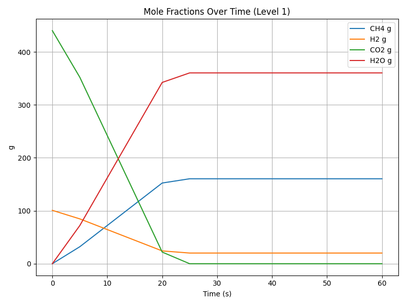
Moles of Reactants and Products Over Time

Starting with 100g of $\text{H}_2$ and 440g of $\text{CO}_2$ we can see that at a constant rate of 0.5 mol/s, the reaction is complete after a bit more than 20 seconds as we run out of $\text{CO}_2$. So at least in the context of this model $\text{CO}_2$ is the limiting reactant and far more $\text{H}_2O$ is produced (360g) than $\text{CH}_4$ (160g). We consume 22g of $\text{CO}_2$, 4g of $\text{H}_2$, and produce 8g of $\text{CH}_4$ and 18g of $\text{H}_2O$ per second for a total of 160g of $\text{CH}_4$ and 360g of $\text{H}_2O$ with around 20g of $\text{H}_2$ left over.

Level 2: Batch Model with Kinetic Rate Law

Level two introduces the Arrhenius equation to calculate the rate constant for the reaction. This increases the complexity of the model but allows more realistic modeling of reaction kinetics. This is similar to the initial $r(t) = r_0$ but we can actually use empirically derived values to calculate the rate constant leading to a more realistic model.

Modeling Rate Kinetics: The Arrhenius Equation

The Arrhenius equation calculates the rate constant $k$—the frequency of successfully reacting collisions per unit concentration (moles per liter) per unit time (seconds). It does this by multiplying the theoretical maximum collision frequency (the pre-exponential factor, $A$) by the exponential of the negative ratio of the activation energy ($E_a$) to the available thermal energy ($RT$).

$$ k(T) = A e^{-\frac{E_a}{RT}} $$

$ k $: rate constant linking rate to concentrations via a rate law. Units depend on overall order; for second-order kinetics they are [L mol$^{-1}$ s$^{-1}$].
$ A $: the pre-exponential factor, representing the theoretical maximum collision frequency when there's no activation energy barrier. It reflects both the frequency and correct orientation of molecular collisions. Its units match those of the rate constant, typically expressed as concentration per unit time [L mol$^{-1}$ s$^{-1}$].
$ E_a $: the activation energy (in Joules per mole, $\text{J/mol}$), representing the minimum energy required for reactants to transform into products.
$ R $: the universal gas constant, equal to 8.314 J/(mol·K). It serves as a scaling factor that relates activation energy and temperature to comparable units.
$ T $: the absolute temperature in Kelvin (K), related directly to the average kinetic energy of the reacting molecules. Higher temperatures increase reaction rates by providing more molecules with sufficient energy to surpass the activation energy barrier.

We can use empirically derived values for the pre exponential factor and activation energy

So we can now write the rate law for the reaction as:

$$ r = k(T)\,C_{\mathrm{CO_2}}\,C_{\mathrm{H_2}}^{\,m} $$

$m$ is the reaction order with respect to $\text{H}_2$. It reflects how strongly the reaction rate depends on the hydrogen concentration. In practice, the value of m isn’t fixed—it’s usually determined experimentally by fitting reaction rate data, and can vary depending on the operating conditions and the catalyst used.

For the concentration of each species we have a system of ODEs that looks like this:

$$\frac{dC_i}{dt} = \nu_i\, r(t)$$

As you can see this is the same as the level 1 model, showing that the only change is the rate law.

Level 3: Plug Flow Reactor Model

In level three we introduce a reactor model: the Plug Flow Reactor. This is a common model used in chemical engineering to design reactors.

Modeling the Plug Flow Reactor (PFR):

The model consists of a series of infinitely small segments of the reactor volume known as 'plugs'. It is an idealized model that assumes no axial mixing between plugs and radial concentration of reactants is assumed to be constant for any given plug. This model shifts our independent variable from time $t$ to space $z$ along the length of the reactor.

$$ \frac{dC_i}{dz} = \frac{\nu_i\, r(z)}{u} $$

Where $u$ is the velocity of the fluid in (m/s), $z$ is the axial position along the length of the reactor, and $r(z)$ is the rate of the reaction at position $z$. So stated simply, the change in concentration of the $i$th species over the length of the reactor is equal to the rate of the reaction at position $z$ divided by the velocity of the fluid.

In modifying the simulation to use the PFR model we can say that the model's inputs are the feed concentrations $C_i(0)$ and velocity $u$. As fluid advances in space by $dz$ species are consumed and produced according to the stoichiometric coefficient $\nu_i$ and the rate law $r(z)$. We solve the ODE along the length of the reactor to get the concentration profile at the outlet.

This model isn't particularly realistic, but it's a good starting point for understanding the PFR model. The methanation reaction in particular suffers from the isobaric, isothermal, and constant velocity assumptions.

Level 4: Molar Flow Rate Model with Pressure and Temperature Variations

Level four removes the assumption of constant temperature, pressure, and velocity. This encourages us to restate the governing equations in terms of the molar flow rates $F_i$ instead of the concentrations $C_i$ removing a circular dependency between the velocity $u$ and the pressure $P$ that would otherwise exist. Here is the new governing equation for the molar flow rates:

$$ \frac{dF_i}{dz} = A \nu_i\, r(z) $$

Where $F_i$ is the molar flow rate of the $i$th species at position $z$, $A$ is the cross-sectional area of the reactor, and $\nu_i$ is the stoichiometric coefficient of the $i$th species.

Given this modification the inputs become the inlet molar flow rates $F_i(0)$ pressure $P(0)$ and temperature $T(0)$.

Modeling Pressure: The Ergun Equation:

Given that methanation is a gas phase reaction it's important to consider how the velocity of the fluid changes along the length due to molar flow of the reactants and products of the reaction. Methanation must also take place in the presence of a catalyst (Ni or Ru are common) and this is often a packed bed of pellets. The presence of the catalyst creates drag of the fluid dropping the pressure and altering its velocity.

The Ergun equation allows us to model the pressure gradient $dP/dz$ as a function of the velocity $u$, the viscosity $\mu$, the density $\rho$ of the fluid as well as the void fraction $\varepsilon$, and the particle diameter $d_p$ of the packed bed.

$$\frac{dP}{dz}=-\Bigg[\frac{150(1-\varepsilon)^2}{\varepsilon^3}\frac{\mu\,u}{d_p^2} \;+\; \frac{1.75(1-\varepsilon)}{\varepsilon^3}\frac{\rho\,u^2}{d_p}\Bigg]$$

Where $dP/dz$ is the pressure per unit length of the packed bed (Pa/m), $\varepsilon$ is the void fraction (porosity) of the packed bed, $\mu$ is the viscosity of the fluid, $\rho$ is the density of the fluid, $u$ is the velocity of the fluid, and $d_p$ is the particle diameter (m) of the packed bed.

The first term on the right-hand side ($\frac{150(1-\varepsilon)^2}{\varepsilon^3}\frac{\mu\,u}{d_p^2}$) represents laminar flow resistance, while the second term ($\frac{1.75(1-\varepsilon)}{\varepsilon^3}\frac{\rho\,u^2}{d_p}$) represents turbulent flow resistance.

It's worth noting that the $u$ is the superficial velocity of the fluid, not the interstitial velocity. The interstitial velocity is the velocity of the fluid through the voids of the packed bed. The superficial velocity is the velocity of the fluid through the entire cross-sectional area of the reactor.

Modeling Temperature: The Energy Balance Equation:

It's also important to consider the energy balance of the reactor. The sabatier reaction is an exothermic reaction, meaning energy (heat) is released as products are formed. This has effects on the local temperature of the reactor. We can model this with an energy balance equation.

$$\frac{dT}{dz}=\frac{-\Delta H_r(T)\,r(z)\,A \;-\; U\,P_w\,[T(z)-T_\infty]}{\,F_\text{tot}(z)\,\bar C_p(z)}$$

Where $\Delta H_r(T)$ is the heat of reaction at temperature $T$, $r(z)$ is the rate of the reaction at position $z$, $A$ is the cross-sectional area of the reactor, $U$ is the overall heat transfer coefficient, $P_w$ is the perimeter of the reactor, $T_\infty$ is the ambient temperature, $F_\text{tot}(z)$ is the total molar flow rate at position $z$, and $\bar C_p(z)$ is the average heat capacity of the fluid at position $z$. Note the negative sign on the heat of reaction indicating that the reaction is exothermic.

Conceptually, the numerator contains the heat of reaction on the left and heat exchange with the wall on the right. The denominator contains the total heat capacity of the fluid at position $z$.

Simulating the PFR

Simulating the PFR to account for variable temperature and pressure requires us to treat some quantities as ODE states $[F_i(z), T(z), P(z)]$ and others as algebraic updates $[F_\text{tot}(z), y_i(z), C_i(z), u(z), \rho(z), r(z)]$. Our ODE states are molar flow rates $F_i(z)$, temperature $T(z)$, and pressure $P(z)$. Total molar flow $F_\text{tot}(z)$, mole fraction $y_i(z)$, concentration $C_i(z)$, velocity $u(z)$, density $\rho(z)$, and reaction rate $r(z)$ are algebraic updates.

Total molar flow $F_\text{tot}(z)$ is calculated as the sum of the molar flow rates of the species at position $z$.

$$ F_\text{tot}(z) = \sum_{i=1}^4 F_i(z) $$

Mole fraction $y_i(z)$ is calculated as the molar flow rate of the $i$th species at position $z$ divided by the total molar flow rate at position $z$.

$$ y_i(z) = \frac{F_i(z)}{F_\text{tot}(z)} $$

Concentration $C_i(z)$ is calculated as the mole fraction of the $i$th species at position $z$: $y_i(z)$, multiplied by the pressure $P(z)$ divided by the universal gas constant $R$ and the temperature $T(z)$.

$$ C_i(z) = y_i(z) \frac{P(z)}{R T(z)} $$

Velocity $u(z)$ is calculated as the total molar flow rate at position $z$ multiplied by the universal gas constant $R$ and the temperature $T(z)$ divided by the cross-sectional area $A$ and the pressure $P(z)$.

$$ u(z) = \frac{F_\text{tot}(z) R T(z)}{A P(z)} $$

Density $\rho(z)$ is calculated as the pressure $P(z)$ multiplied by total molar mass of the mixture $\bar M(z)$ divided by the universal gas constant $R$ and the temperature $T(z)$.

$$ \bar M(z) = \sum_{i=1}^4 y_i(z)\,M_i $$

$$ \rho(z) = \frac{P(z)\,\bar M(z)}{R\,T(z)} $$

Reaction rate is the same as the level 2 model.

$$ r(z) = k(T)\,C_{\mathrm{CO_2}}\,C_{\mathrm{H_2}}^{\,m} $$

Level 4 Results

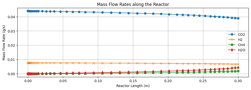
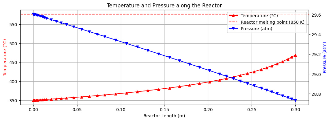
Moles of Reactants and Products Over Time

The results of the level 4 model are shown above. We can see a obvious rise in $\text{CH}_4$ and $\text{H}_2O$ product flow and temperature as we move from the inlet to the outlet of the reactor demonstrating the exothermic nature of the reaction.

Residence time ≈ 0.054 s
Outlet molar flow of CO2: 0.88 mol/s, 0.038832 g/s, 2.329937 g/min, 139.796235 g/h
Outlet molar flow of H2: 3.33 mol/s, 0.006712 g/s, 0.402706 g/min, 24.162348 g/h
Outlet molar flow of CH4: 0.12 mol/s, 0.001887 g/s, 0.113233 g/min, 6.793978 g/h
Outlet molar flow of H2O: 0.24 mol/s, 0.004239 g/s, 0.254315 g/min, 15.258895 g/h
Outlet stream percentage of CO2: 19.33%
Outlet stream percentage of H2: 72.94%
Outlet stream percentage of CH4: 2.58%
Outlet stream percentage of H2O: 5.15%

This model, while more complex, is still a simplification of the real world. It doesn't account for the effectiveness of the catalyst, non-ideal gas behavior, side reactions, and other factors that would affect the reaction rate and product yield. However, it's a good starting point for understanding the methanation reaction and the challenges involved in modeling it. I plan to extend the model to include these factors in future posts.

Level 5: Adding Reversibility and Side Reactions

In a real world methanation reactor there are far more reactions occurring than just the $\text{CO}_2$ methanation reaction. These include the water-gas shift and $\text{CO}$ methanation. We will also want to account for reversibility of our reactions. For clarity let's write out each reaction we want to model.

$$ \text{$\text{CO}_2$ methanation} \quad \text{CO}_2 + \text{4H}_2 \rightleftharpoons \text{CH}_4 + \text{2H}_2O \quad (1) $$

$$ \text{CO methanation} \quad \text{CO} + \text{3H}_2 \rightleftharpoons \text{CH}_4 + \text{H}_2O \quad (2) $$

$$ \text{Water-gas shift} \quad \text{CO} + \text{H}_2O \rightleftharpoons \text{CO}_2 + \text{H}_2 \quad (3) $$

We can represent these for our simulation in a matrix form where each row is species and each column is a reaction like so:

$$ \nu = \begin{bmatrix} -1 & 0 & 1 \ -4 & -3 & 1 \ 1 & 1 & 0 \ 2 & 1 & -1 \ 0 & -1 & -1 \ \end{bmatrix} $$

So column 1 $[-1, -4, 1, 2, 0]$ represents the stoichiometric coefficients of reaction 1: the sabatier reaction ($\text{CO}_2$ methanation). Whereas row 1 $[-1, 0, 1]$ represents the stoichiometric coefficients of species 1: $\text{CO}_2$ in each reaction*.

*These would be column 0 and row 0 in the code due to zero based indexing.

This arrangement requires we modify our energy balance equation to account for the heat of reaction of each reaction.

$$ \frac{dT}{dz} \;=\; \frac{\displaystyle A \sum_{j=1}^{R} !(-\Delta H_j(T))\, r_j(z) \;-\; U P_w (T - T_\infty)}{F_\text{tot}\,\bar C_p} $$

Where $\Delta H_r(T)_j$ is the heat of reaction for the $j$th reaction at temperature $T$, $r_j$ is the rate of the $j$th reaction at position $z$, and $R$ is the number of reactions.

The pressure drop $\frac{dP}{dz}$ is the same as the level 4 model.

Reaction Rates and Equilibrium Constants

We also need to formulate reaction rates for each reaction. For the $j$th reaction we can model the reaction rate as follows:

$$ r_j(z) = k_j(T) \phi_j(a) (1 - \frac{Q_j(a)}{K_j(T)})$$

Where $r_j(z)$ is the rate of the $j$th reaction at position $z$. $k_j(T)$ is the rate constant for the $j$th reaction at temperature $T$. (Arrhenius equation) $\phi_j(a)$ is the forward activity dependence for the $j$th reaction. This is similar to the power law approach we've shown before in that it is an empirically derived value.

For CO2 methanation we can model the forward activity dependence as follows: $$ \phi_1(a) = a_{\mathrm{CO_2}}^{\alpha_1} a_{\mathrm{H_2}}^{\beta_1} $$ Where $\alpha_1$ and $\beta_1$ are the empirically fitted values for each species in reaction 1. $a_i$ is the activity of the $i$th species. Using ideal gas assumptions: $$ a_i = \frac{y_i(z) P(z)}{P^\circ} $$

Where $y_i(z)$ is the mole fraction of the $i$th species at position $z$ as a percentage. $P^\circ$ is the standard pressure of 1 bar. $P(z)$ is the pressure at position $z$.

$Q_j(a)$ is the reaction quotient for the $j$th reaction. This uses stoichiometric coefficients.

$$ Q_j(a) = \prod_{i}{a_i^{\nu_{i,j}}} $$

or for CO2 methanation:

$$ Q_1 = \frac{a_{\mathrm{CH_4}} a_{\mathrm{H_2O}}^2}{a_{\mathrm{CO_2}} a_{\mathrm{H_2}}^4} $$

$K_{pj}(T)$ is the equilibrium constant for the $j$th reaction at temperature $T$. This is the ratio of product activities to reactant activities and essentially serves as a measure of the extent to which the reaction proceeds towards or away from equilibrium (where the reaction rate is zero and both forward and reverse rates are equal). At equilibrium $r_j = 0$ and $Q_j(a) = K_{pj}(T)$.

$$ K_{pj}(T) = e^{-\frac{\Delta_{G_{r_j}^\circ(T)}}{RT}} $$

With this we can write out the ODE for molar flow rates like so:

$$ \frac{dF_i}{dz} = A (\nu \cdot r(z))_i $$

Level 6: Catalytic Surface Modeling

Level six introduces a more complete treatment of the surface phenomena at the catalyst. Langmuir-Hinshelwood (L-H) kinetics captures the adsorption and desorption of the reactants and products on the catalyst surface. The essence of this model is that species absorb onto the catalyst and either amalgamate or dissociate to form surface species at a finite number of sites. I'll first describe the mechanistic details of the process and then discuss the modeling implications.

Adsorption

$CO_2$ gas molecules from the input stream can come into contact with the Ni catalyst. Depending on the local thermal conditions the $CO_2$ can undergo adsorption onto the catalyst in several different ways. The most desirable from our perspective would be a monodentate adsorption where the Carbons empty pi bonds are filled by the available electrons in the d orbital of the Ni atom. This is a likely occurrence at higher temperatures (>300 C), however, at lower temperatures the more energetically favorable outcome is a bidentate adsorption where one or both of the Oxygen atoms bond to the catalyst.

$H_2$ gas molecules from the input stream undergo a similar adsorption process, but $H_2$ gas dissociates almost immediately upon adsorption. The dissociated $H$ atoms having a relatively small atomic mass are far more free to move about on the surface of the catalyst. This freedom of movement works to our advantage.

Dissociation

With the occurrence the favorable monodentate case, the shifting of the electrons in the molecule weakens the Carbon's bonds to the Oxygen atoms, thereby decreasing the activation energy needed for the Oxygen to dissociate. The dissociation of one or both of the Oxygen atoms from the Carbon atom is once again a function of the local thermal conditions. In addition to this, dissociation is a function of the local geometry of the catalyst. Terraces, steps, and edges can all effect the probability of dissociation. In addition to these conditions high coverage rates of adjacent active sites can hinder dissociation through steric hindrance. It is often the case that the Dissociation the the Oxygen atoms happens as separate steps and not simultaneously. Dissociated Oxygen atoms typically reside as surface species strongly bound to the catalyst.

Dissociated Oxygen atoms freed from their bonds to Carbon and undergo adsorption. When a freely moving hydrogen encounters and Oxygen atom hydrogenation is a likely occurrence. After two hydrogenations $H_2O$ is formed and will freely undergo desorption from the catalyst.

Hydrogenation

When the surface Carbon atom is visited by a traveling Hydrogen atom a hydrogenation is likely to occur. After three of these $CH_3$ is formed and is only left singly bound to the Ni catalyst. One more subsequent hydrogenation event and $CH_4$ is formed. $CH_4$ having all the valence electrons engaged with Hydrogen atoms is no longer chemically bound to the catalyst and can easily undergo desorption. Intermediate hydrogenation steps have different adsorptions strengths. $CH$ and $CH_2$ are very strongly bound to the catalyst.

Desorption

Surface species of $CH_4$ are only bound by weak Van der Waals forces and will readily desorb from the catalyst.

At this point we face a choice. Should we keep axial position $z$ as the independent variable or should we switch to catalyst mass $m$? For the sake of simplicity I'll keep $z$ as the independent variable. Perhaps in a future post we can explore the use of catalyst mass as the independent variable.

Langmuir-Hinshelwood

While I did explore tracking each surface species independently using an internal non-linear solver, it was a bit of a mess and frankly I think too large of a complexity step for what I'm shooting for here. So I'll be using the single site Langmuir-Hinshelwood form. In this form we assume there is a single rate-limiting step that determines the overall reaction rate. Each gas has an equilibrium constant defining how much of the gas will adsorb to the surface. All reactants and products compete for a finite number of surface sites. Empty spots shrink as they are filled and only remaining empty spots are available for the rate-limiting step. We can define empty spots as $\theta_*$ and describe this as follows:

$$ \theta_* = \frac{1}{1 + \sum_i \tilde K_i a_i} $$

We can compute reaction rate for $CO_2$ methanation using the following equation.

$$ r = k(T)\,\frac{\tilde K_{CO_2}a_{CO_2}\,\tilde K_{H_2}a_{H_2}^{2}}{\big(1 + \tilde K_{CO_2}a_{CO_2} + \tilde K_{H_2}a_{H_2} + \tilde K_{CO}a_{CO} + \tilde K_{H_2O}a_{H_2O}\big)^m}\,\Big(1 - \tfrac{Q}{K_p(T)}\Big). $$

$$ Q = \frac{a_{CH_4}a_{H_2O}^2}{a_{CO_2}a_{H_2}^4} $$

Where the numerator is the products of activities and adsorption constants for the reactant species. The denominator represents the competition for the surface sites and is the sum of the products of partial pressures and adsorption constants for other species present. $m$ is the vacant site order, expressing the number of vacant sites required by the rate-limiting step. The result of this is multiplied by a driving force term $(1 - \tfrac{Q}{K_p(T)})$ ensuring the system respects thermodynamic equilibrium. Where $Q$ is the reaction quotient and $K_p(T)$ is the equilibrium constant at temperature $T$.

$CO$ methanation: $$ r = k(T)\,\frac{\tilde K_{CO}a_{CO}\,\tilde K_{H_2}a_{H_2}^{3}}{\big(1 + \tilde K_{CO_2}a_{CO_2} + \tilde K_{H_2}a_{H_2} + \tilde K_{CO}a_{CO} + \tilde K_{H_2O}a_{H_2O}\big)^m}\,\Big(1 - \tfrac{Q}{K_p(T)}\Big). $$

$$ Q = \frac{a_{CH_4}a_{H_2O}}{a_{CO}a_{H_2}^3} $$

Water-gas shift reaction: $$ r = k(T)\,\frac{\tilde K_{CO}a_{CO}\,\tilde K_{H_2O}a_{H_2O}}{\big(1 + \tilde K_{CO_2}a_{CO_2} + \tilde K_{H_2}a_{H_2} + \tilde K_{CO}a_{CO} + \tilde K_{H_2O}a_{H_2O}\big)^m}\,\Big(1 - \tfrac{Q}{K_p(T)}\Big). $$

$$ Q = \frac{a_{CO_2}a_{H_2}}{a_{CO}a_{H_2O}} $$

Now I will introduce a couple new parameters regarding the catalyst. $\Gamma$ and $a_{\text{cat}}$.

$\Gamma$ is the surface site density. This is the number of surface sites per unit area of catalyst in units of $\text{mol sites} * m^{-2}$.

$a_{\text{cat}}$ is the catalyst surface area per unit volume of reactor in units of $m^2_{cat}/m^3_{bed}$.

We can use these to compute the volumetric reaction rate for each reaction. $$ \dot{R}^{vol} = a_{\text{cat}}\,\Gamma\,r $$

Next we can compute the net production rate $\omega_i$ for each species. $$ \omega_i = \sum_{s=1}^{S} \nu_{i,s}\,\dot R_s^{(\text{vol})} $$

And we can describe the molar flow using a familiar ODE. $$ \frac{dF_i}{dz} = A \omega_i $$

Polymerization and Catalyst Poisoning

Low $H_2$ availability, high temperatures, carbon rich conditions, or slow hydrogenation can cause the surface Carbon to undergo polymerization and form graphitic structures on the catalyst. This will semi-permanently bind the carbon to the surface making the site unusable for further reactions. If enough of these event processes termed coke formation occur it can poison the catalyst and affect the output yields. We can model coke formation by adding a pseudo species $\theta_{C}$ to the system that will adsorb to the catalyst surface and prevent further reactions.

So far, this model assumes every molecule can instantly reach every active site and that the catalyst is uniformly at reactor temperature. Reality is a bit harsher: molecules must diffuse through pores in the catalyst body, heat builds up locally, and an actual reactor isn’t a perfect PFR without axial dispersion or radial gradients. Perhaps in a future post I can explore these effects, but I think I've covered enough for now.

Level 6 Results

Appendix:

Code for level 4

UNIVERSAL_GAS_CONSTANT = 8.314462618 # J/mol K

# Reactor parameters (PFR)
REACTOR_LENGTH = 0.3 # m
REACTOR_DIAMETER = 0.045 # m
CROSS_SECTIONAL_AREA = np.pi * (REACTOR_DIAMETER / 2)**2 # m^2 (circular)
PERIMETER = np.pi * REACTOR_DIAMETER # m (circular)

# Packed bed parameters
POROSITY = 0.4 # unit-less
PARTICLE_DIAMETER = 0.01 # m

# Energy balance parameters
HEAT_TRANSFER_COEFFICIENT = 150 # W/m^2 K
TEMPERATURE_AMBIENT = 298.15 # K
VISCOSITY = 2.0e-5 # Pa s (viscosity of fluid) [constant, could be a function of temperature]

SPECIES_MASSES = np.array([
    44.0095e-3, # co2, kg/mol
    2.01588e-3, # h2, kg/mol
    16.0425e-3, # ch4, kg/mol
    18.01528e-3 # h2o, kg/mol
])

SPECIES_HEAT_CAPACITIES = np.array([
    37.1, # co2, J/mol/K
    28.8, # h2, J/mol/K
    35.7, # ch4, J/mol/K
    34.0 # h2o, J/mol/K
])

STOICHIOMETRIC_COEFFICIENTS = np.array([
    -1, # co2
    -4, # h2
    1, # ch4
    2 # h2o
])

# Kinetics
PRE_EXPONENTIAL_FACTOR = 1.0e4 # m^3/(mol·s)
ACTIVATION_ENERGY = 80e3 # J/mol
MH2 = 1.0 # order w.r.t. H2
DELTA_ENTHALPY_REACTION = -165e3 # J/mol

def rate_constant_arrhenius(temperature):
    return PRE_EXPONENTIAL_FACTOR * np.exp(-ACTIVATION_ENERGY / (UNIVERSAL_GAS_CONSTANT * temperature))

def mixture_properties(molar_flow_rates, temperature, pressure):
    # F_tot, y_i, C_i, bar M, rho, u
    total_molar_flow_rate = np.sum(molar_flow_rates) # F_tot(z)
    total_molar_flow_rate = max(total_molar_flow_rate, 1e-12) # avoid division by zero

    species_mole_fractions = molar_flow_rates / total_molar_flow_rate # y_i(z)
    species_concentrations = species_mole_fractions * (pressure / (UNIVERSAL_GAS_CONSTANT * temperature)) # C_i(z)
    mixture_molar_mass = np.dot(species_mole_fractions, SPECIES_MASSES) # bar M(z)
    mixture_density = (pressure * mixture_molar_mass) / (UNIVERSAL_GAS_CONSTANT * temperature) # rho(z)

    superficial_velocity = (total_molar_flow_rate * UNIVERSAL_GAS_CONSTANT * temperature) / (CROSS_SECTIONAL_AREA * pressure) # u(z)

    return total_molar_flow_rate, species_mole_fractions, species_concentrations, mixture_molar_mass, mixture_density, superficial_velocity

def ergun_dp_dz(velocity, density):
    laminar_flow_resistance = ((150 * (1 - POROSITY)**2) / (POROSITY**3)) * ((VISCOSITY * velocity) / (PARTICLE_DIAMETER**2))
    turbulent_flow_resistance = ((1.75 * (1 - POROSITY)) / (POROSITY**3)) * ((density * velocity**2) / (PARTICLE_DIAMETER))
    return -(laminar_flow_resistance + turbulent_flow_resistance)

def energy_balance_dt_dz(total_molar_flow_rate, reaction_rate, temperature, heat_capacity_of_mixture):
    heat_of_reaction = -DELTA_ENTHALPY_REACTION * reaction_rate * CROSS_SECTIONAL_AREA
    heat_exchange_w_environment = -HEAT_TRANSFER_COEFFICIENT * PERIMETER * (temperature - TEMPERATURE_AMBIENT)
    heat_capacity_of_fluid = total_molar_flow_rate * heat_capacity_of_mixture
    return (heat_of_reaction + heat_exchange_w_environment) / heat_capacity_of_fluid

def calculate_reaction_rate(rate_constant, species_concentrations):
    # r = k * C_CO2 * C_H2^mH2
    return rate_constant * species_concentrations[0] * species_concentrations[1]**MH2

def pfr_rhs(z, y):
    molar_flow_rates = y[:4] # mol/s (molar flow rates)
    temperature = y[4] # K (temperature)
    pressure = y[5] # Pa (pressure)

    # Unpack mixture properties
    (total_molar_flow_rate, # mol/s
     species_mole_fractions, # unit-less
     species_concentrations, # mol/m^3
     mixture_molar_mass, # kg/mol
     mixture_density, # kg/m^3
     superficial_velocity # m/s
    ) = mixture_properties(molar_flow_rates, temperature, pressure)

    # Reaction rate
    rate_constant = rate_constant_arrhenius(temperature)
    reaction_rate = calculate_reaction_rate(rate_constant, species_concentrations) # mol/m^3/s

    # Energy balance
    df_dz = CROSS_SECTIONAL_AREA * STOICHIOMETRIC_COEFFICIENTS * reaction_rate # mol/s
    dp_dz = ergun_dp_dz(superficial_velocity, mixture_density) # Pa/m
    heat_capacity_of_mixture = np.dot(species_mole_fractions, SPECIES_HEAT_CAPACITIES) # J/mol/K (heat capacity of mixture) [c_p(z) = sum(y_i(z) * c_p_i(z))]
    dt_dz = energy_balance_dt_dz(total_molar_flow_rate, 
                                 reaction_rate,
                                 temperature,
                                 heat_capacity_of_mixture) # K/m    
    return np.array([df_dz[0], df_dz[1], df_dz[2], df_dz[3], dt_dz, dp_dz], dtype=float)

# Initial conditions
F0_CO2 = 1.00 # mol/s
F0_H2  = 3.80 # mol/s
F0_CH4 = 0.0 # mol/s
F0_H2O = 0.0 # mol/s
T0 = 623.0  # K
P0 = 3.0e6  # Pa

y0 = np.array([F0_CO2, F0_H2, F0_CH4, F0_H2O, T0, P0], dtype=float)

# Safety events
def stop_negative_flows(z, y): return np.min(y[0:4])
stop_negative_flows.terminal = True
stop_negative_flows.direction = -1

# Aluminum melting point (6061)
def stop_high_temperature(z, y): return y[4] - 850.0
stop_high_temperature.terminal = True
stop_high_temperature.direction = 1

z_span = (0.0, REACTOR_LENGTH)

sol = solve_ivp(
    lambda z, y: pfr_rhs(z, y),
    z_span,
    y0,
    method='BDF',
    rtol=1e-6,
    atol=1e-9,
    events=[stop_negative_flows],
    dense_output=True
)

sol

Weapons Grade Bolognium